Guide · Updated September 2026
Say you have two columns — maybe last week’s inventory list and this week’s — and need to know what changed. Here are three ways to compare them, roughly in order of how much Excel knowledge they require.
Compare Two Columns in Excel: Quick Answer
Excel has no single command to compare two columns directly. The fastest reliable method: copy each column into a free browser-based comparison tool and read four results at once — items only in column A, only in column B, shared values, and the combined set — without writing or maintaining a COUNTIF or MATCH formula.
Method 1: Conditional formatting
Select both columns, then Home → Conditional Formatting → Highlight Cells Rules → Duplicate Values. Choose “Unique” instead of “Duplicate” to highlight items that don’t match. See Microsoft’s conditional formatting documentation for the full rule options. This works well for a quick visual scan but doesn’t separate “only in column A” from “only in column B” — both get flagged the same color.
Method 2: A COUNTIF/MATCH formula
In a helper column next to List A, use COUNTIF:
=IF(COUNTIF(B:B, A2)=0, "Missing from B", "Match")
Fill down, then filter for “Missing from B.” Repeat in reverse (COUNTIF against A) to find what’s missing from A. This gives you a real difference set, but it’s two separate formulas, and things like extra spaces or mismatched casing will silently break the match unless you wrap both sides in TRIM() and LOWER().
Method 3: Paste both columns into a comparison tool
Copy column A into List 1 and column B into List 2in a browser-based list comparison tool. You get all four differences at once — only in A, only in B, shared, and combined — with case-sensitivity and whitespace handling as toggles instead of nested formulas, and nothing leaves your browser.
Which method to use
- One-off visual check on a small range → conditional formatting.
- Need the difference as data you can filter or export → formulas, if you’re comfortable maintaining them.
- Want a clean result you can copy out immediately, with duplicates and case handled for you → paste into a comparison tool.
Worked example
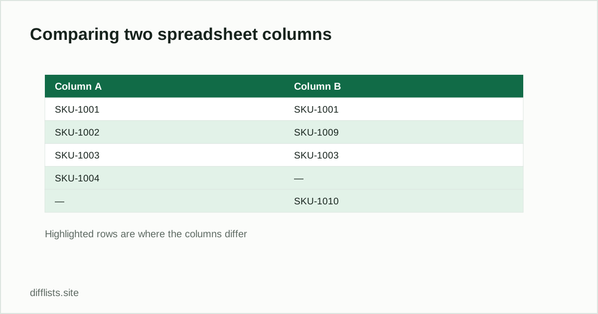
Say column A holds last week’s product SKUs and column B holds this week’s:
| Column A (last week) | Column B (this week) |
|---|---|
| SKU-1001 | SKU-1001 |
| SKU-1002 | SKU-1009 |
| SKU-1003 | SKU-1003 |
| SKU-1004 | — |
| — | SKU-1010 |
Paste column A into List 1 and column B into List 2. The result: Only in List 1 is SKU-1002 and SKU-1004 (removed or discontinued this week). Only in List 2 is SKU-1009 and SKU-1010 (newly added). Intersectionis SKU-1001 and SKU-1003 (unchanged). No COUNTIF, no helper column — the same five results a formula would eventually produce, in one paste.
For the Google Sheets equivalent, see How to Compare Two Lists in Google Sheets.
Paste your two columns and compare instantly.
Open the toolFrequently asked questions
How do I compare two columns in Excel for differences?
Use Home → Conditional Formatting → Highlight Cells Rules → Duplicate Values (choose Unique) for a quick scan, or paste both columns into a comparison tool for a full difference list.
What formula compares two Excel columns?
=IF(COUNTIF(B:B,A2)=0,"Missing from B","Match") flags values in column A that don't appear anywhere in column B.
Why does my COUNTIF formula miss obvious matches?
Extra spaces or mismatched letter case silently break COUNTIF matches — wrap both sides in TRIM() and LOWER(), or use a comparison tool that normalizes both automatically.
Can I compare two columns without writing a formula?
Yes — copy each column and paste it into a browser-based list comparison tool to get differences, matches, and a combined list without any formulas.
Can I compare two columns across two different Excel workbooks?
Yes — copy the column from each workbook the same way you would within one file; the comparison only needs the pasted values, not which file they came from.
Why does my column comparison miss matches that look identical?
Trailing spaces, mismatched capitalization, or a hidden apostrophe forcing text formatting on numbers are the usual culprits — wrap COUNTIF in TRIM()/LOWER(), or use a comparison tool that normalizes both automatically.