Guide · Updated September 2026
Google Sheets: Compare Two Lists in One Paste
Google Sheets has no single built-in command for this, so most people reach for a MATCH or ISNA formula in a helper column, or conditional formatting for a quick visual scan. The faster route: paste both columns into a free browser-based tool and get every match, difference, and combined set instantly, with no formulas to clean up afterward.
Method 1: ISNA + MATCH formula
In a blank column next to List A, use MATCH:
=IF(ISNA(MATCH(A2, B:B, 0)), "Not in B", "Match")
This flags every A2 value that has no match anywhere in column B. Copy the formula down the column, then use Data → Create a filterto isolate the “Not in B” rows. Swap the ranges to check the reverse direction.
Method 2: Conditional formatting
Select both ranges, open Format → Conditional formatting, and use a custom formula like =COUNTIF($B$:$B, A1)=0to highlight cells in A with no match in B — see Google’s conditional formatting rules documentation for the full set of options. Good for a quick visual pass over a small sheet; harder to read once a list runs into the thousands of rows.
A faster way: paste both columns into a comparison tool
Select column A, copy, and paste into List 1; do the same for column B into List 2. You immediately get everything only in A, only in B, what’s shared, and the full combined set — no helper columns, no filters to remember to remove afterward. Toggle case sensitive if your sheet uses codes where case matters, and natural sort if you want numeric IDs ordered correctly instead of alphabetically.
Which is better?
If the comparison needs to live inside the spreadsheet — recalculating as the sheet updates — formulas are the right call. For a one-off “what changed between these two exports” question, pasting into a dedicated comparison tool is faster and easier to read.
Worked example
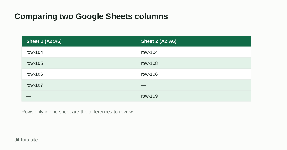
Two sheets tracking the same order IDs, one week apart:
| Sheet 1, column A | Sheet 2, column A |
|---|---|
| row-104 | row-104 |
| row-105 | row-108 |
| row-106 | row-106 |
| row-107 | — |
| — | row-109 |
Copy each column into a list panel and compare. row-104 and row-106 match (intersection); row-105 and row-107 dropped out of Sheet 2 (only in List 1); row-108 and row-109 are new to Sheet 2 (only in List 2). No ISNA/MATCH formula to write or clean up afterward.
Comparing Excel columns instead of Google Sheets? See comparing two Excel columns for the Excel-specific formulas.
Skip the formulas and compare your columns now.
Open the toolFrequently asked questions
How do I compare two Google Sheets for differences?
Use =IF(ISNA(MATCH(A2,B:B,0)),"Not in B","Match") in a helper column, or paste both columns into a comparison tool for the full difference set without formulas.
How do I find duplicates in Google Sheets between two columns?
Compare the two columns and read the Intersection result — every value that appears in both columns is a duplicate between them.
Does the formula method update automatically?
Yes — a MATCH-based formula recalculates as the sheet changes, which a one-off paste into an external tool won't do.
What if my Google Sheets columns use different letter casing?
MATCH is case-insensitive by default in Sheets. If you need exact case matching, use EXACT() in the formula, or toggle case sensitivity on in a comparison tool.
Can Google Sheets compare two lists automatically, without formulas?
Not natively inside a sheet — but you can skip formulas entirely by pasting both columns into a free browser-based comparison tool, which returns every difference, match, and combined set in one pass.
Is there a Google Sheets add-on to compare two lists?
A few exist in the Add-ons store, but they require granting a third-party add-on access to your sheet. A MATCH/ISNA formula or an external comparison tool gets the same result without that permission.